|
|
|
|
|
|---|
|
Pacific northwest coast
|
25%
|
47%
|
17%
|
|
Gulf Coast
|
59%
|
40%
|
67%
|
|
East coast
|
7%
|
7%
|
2%
|
|
Other
|
9%
|
6%
|
13%
|
Source: Authors’ analysis based on USDA (2015), Grain Transportation Report – February 12, https://www.ams.usda.gov/services/transportation-analysis/gtr/archive-2015 (accessed 25 Jan. 2017).
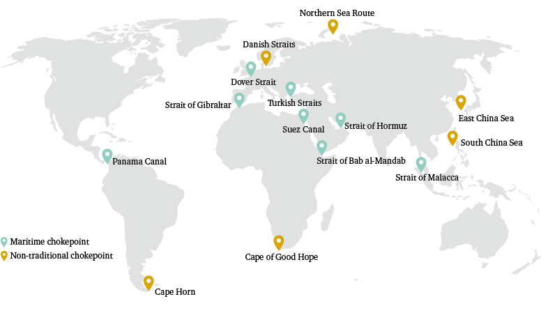
Each region-to-region routing assumption is stored within a two-dimensional array of 1,766 rows (representing every possible region-to-region flow in the database), and 14 fields (representing the eight maritime chokepoints deemed of global strategic importance, plus the Danish Straits, Cape of Good Hope, Cape Horn, Northern Sea Route, South China Sea and East China Sea). Trade flows attributed to ‘areas not elsewhere specified’ in the CHRTD are not assigned a routing assumption in our model.
Methodological limitations
As the first tool of its kind, the CH-MAT includes a number of assumptions and limitations which warrant further probing if the tool’s accuracy and robustness are to be strengthened. Below, we briefly outline these and identify priorities for future research.
Assumptions
On the basis of an extensive literature review and a series of conversations with maritime industry experts, we make the assumption that all grain trade is transported by dry bulk vessels. This is because, while the use of containers in the transport of grain is increasing, available evidence suggests that containerized shipments as a share of total shipments remain low. Our routing assumptions therefore imply single point-to-point voyages. If liner routes were also considered, our approach to region-to-region routing assumptions (based on the distance and shipping time between major trade hubs in region x and region y) might no longer be valid; liner vessels would likely call at other ports en route – picking up or dropping off grain shipments from other trading partners – rather than steaming directly from region x to region y.
Furthermore, the CH-MAT does not account for the movement of vessels empty of cargo. This is because the underlying data for the CH-MAT consist of bilateral trade data rather than port throughput data. Taking only cargo-carrying vessels into account makes sense when assessing the strategic importance of certain routes to food security; in the case of a major blockage to the Panama Canal, for instance, vessels carrying grain shipments, not those that are empty, will be of concern to the food security community. But as empty vessels can also be used in identifying potential points of congestion, their omission from our analysis may lead to an underestimate of usage levels at certain chokepoints or along certain trade routes.
We apply to fertilizer flows the same set of routing assumptions as those developed for grain flows. Having consulted available data on fertilizer shipments to and from major consumers and producers, we are confident that this approach is valid. However, further analysis of the specific patterns of fertilizer trade and of specialized fertilizer-handling terminals would be needed to be sure that no important differences between fertilizer and grain trading patterns have been missed.
Where both maritime and overland trade routes exist between region x and region y and are of comparable distance, we assume that the maritime route will be taken. The exceptions are where seaborne shipments would imply a significant detour: for example, in the case of trade between landlocked countries in Central Asia.
Limitations
In developing our approach to the CH-MAT, we faced a number of challenges arising from poor data availability. Very little analysis has been undertaken of the seaborne movement of grain and/or fertilizer; and while there exists a relatively rich body of literature on global transport networks and patterns of international maritime trade, the idiosyncrasies of shipping data are such that commodity-specific analysis is extremely difficult.
AIS data distinguish between vessel types, for example, but do not detail the cargo carried by any given vessel. Apps such as MarineTraffic allow users to follow the movement of a particular dry bulk carrier but do not indicate the nature of the dry bulk cargo on board; as such, it is not possible to distinguish between coal shipments and wheat shipments, for example. And while rudimentary data – the vessel type and forecast route, for example – are open-access, further details such as the previous and next ports of call are behind a pay wall and therefore likely to be unavailable to many civil society and public actors.
The quality and availability of national data on port capacity, export flows and import flows are extremely variable. Some countries (such as the US and Saudi Arabia) collect and make public fine-grained data on port capacity and throughput, sometimes broken down by commodity type. Others differentiate only between container shipments and dry bulk shipments. Turkey, for example, reports on dry bulk throughput at its ports, but does not distinguish between grain and other dry bulk such as coal and sand. Other countries (such as the Pacific Island states) have little or no open-access data on import and export shipments, let alone statistics for individual port areas.
Consistency in port throughput data across countries is further limited by discrepancies in reporting. While certain countries report in weight-in-tonnage, others report in value-in-currency; and, while certain countries are consistent in their annual reporting, others provide data on an ad hoc basis. We apply consistent rules when selecting data for use in the CH-MAT – data in weight are preferred over data in value wherever possible; the most recent data available in the period 2010–16 are always used – but discrepancies certainly remain.
Finally, the use of bilateral trade data itself implies certain limitations in analysing the patterns of trade in grain. Trade data are reported only annually, and as such the CH-MAT estimates aggregate chokepoint throughput volumes on a yearly basis. This masks important seasonal fluctuations in the export and import of grain; peak flows from South America during the soybean harvest season are balanced out by yearly lows earlier in the cropping cycle, for instance. While a valuable indication of port areas of systemic interest, the CH-MAT therefore offers little basis for capturing periods of relatively high risk when a major disruption to Brazil’s southern ports could, for example, have a disproportionately large impact on global soybean supply.
Review
A number of maritime industry experts and food security analysts provided valuable feedback on our approach to the project since its inception in early 2015. In the summer of 2016, we undertook a more formal process of peer review through which we presented the key steps, assumptions and limitations of the CH-MAT. The reviewers were Dr Tristan Smith (University College London Energy Institute), Dr Michael Traut (University of Manchester Tyndall Centre) and Dr Conor Walsh (University of Manchester Tyndall Centre). We are extremely grateful to these reviewers for their feedback and guidance. However, we remain solely responsible for the development of the CH-MAT and for any errors it may contain. We welcome feedback on how this important tool may be improved and expanded in the future.
A1.2 Chatham House Resource Trade Database (CHRTD)
Richard King, Felix Preston and Siân Bradley
The Chatham House Resource Trade Database (CHRTD) is a repository of statistics on bilateral trade in natural resources between more than 200 countries and territories. The database includes the monetary values and masses of trade in over 1,350 different types of natural resources and resource products, including agricultural, fishery and forestry products, fossil fuels, metals and other minerals, and pearls and gemstones. It contains raw materials, intermediate products and by-products.
Dealing with complexity
Bilateral statistics are critical to understanding global resource trade, but existing data are often difficult to access and use. The original data source for the CHRTD is the International Merchandise Trade Statistics (IMTS). IMTS data are collected by national customs authorities and compiled into the United Nations Commodity Trade Statistics Database (UN Comtrade) by the United Nations Statistics Division. UN Comtrade utilizes three distinct trade classification systems: the Harmonized Commodity Description and Coding System (HS), the Standard International Trade Classification (SITC), and Broad Economic Categories (BEC). Of these, the CHRTD employs the HS taxonomy (1996 revision), which assigns HS codes to all forms of traded goods in a hierarchical structure (two-, four- and six-digit codes respectively represent commodity chapters, headings and subheadings).
Across the resource landscape alternative repositories of trade data are available, but these do not offer the breadth and depth of analysis that UN Comtrade permits. For example:
- Data from the United Nations Conference on Trade and Development (UNCTAD) have the greatest temporal availability, with some aggregate categories dating back to 1948, but even recent series lack commodity-level (six-digit HS code) detail.
- The FAO provides comprehensive bilateral trade data for agriculture, forestry, fisheries and aquaculture, but not for other resource domains. Much of the available data share the same origins as UN Comtrade data and are not necessarily more accurate.
- The USDA Global Agricultural Trade System (GATS) is similarly domain-constrained and focuses on US trading partners. Similarly, the European Commission’s EUROIND database covers only trade with and between EU countries.
- The IEA provides comprehensive energy balance and energy flow statistics, but trade statistics are limited to gas flows within and to Europe.
- US EIA data include national energy consumption, production, and import and export statistics, but lack bilateral detail.
- The world oil and gas databases developed by the Joint Organisations Data Initiative (JODI-Oil and JODI-Gas) were developed as transparency tools rather than trade databases. Unlike other databases, JODI does not adjust reported figures or substitute missing figures, so coverage is incomplete.
- Commercial sources such as the BP Statistical Review of World Energy provide comprehensive energy trade data, but no bilateral dimension.
UN Comtrade is therefore arguably the most comprehensive source of merchandise trade statistics available; volumetric and monetary value data are catalogued under more than 5,000 HS codes, and the monetary values of trades are available as far back as 1962. However, it does present several challenges for users focusing on resource trade, which the CHRTD and Chatham House’s resourcetrade.earth site address:
- The HS system is not easy to use. Its nomenclature has evolved historically as a pragmatic and comprehensive industrial taxonomy for the broad range of internationally traded goods.
- The scale hinders simple queries: with over 3 billion trade records since 1962, finding the right data is not always easy and the size of data queries can be difficult to manage.
The IMTS data are of variable quality: missing data, trade mispricing, unreported and illegal trade, and general mistakes and inconsistencies all cast doubt over the reliability of certain reported trade flows.
The presence of between one and four data points for every trade flow complicates use: both exporters and importers are expected to report trade values and trade masses. If these records are incomplete or do not correspond with one another, there may be uncertainties about the reliability of data and/or about which reporter is the most authoritative.
Introducing clarity
The CHRTD reorganizes data around natural resources. As the IMTS and HS systems contain all types of traded goods – including manufactured goods – analysing natural resource trade flows in UN Comtrade typically requires amalgamating a variety of HS codes. The difficulty of this varies: products that have a long history of being traded extensively are captured in greater detail than those that are traded less frequently. For example, there is a single HS code associated with rare-earth elements, but several hundred codes assigned to steel and steel products. The CHRTD overcomes this problem by selecting over 1,350 HS codes that are identifiable as raw materials or relatively undifferentiated intermediate products, and by grouping them by resource type. For example, copper ores and concentrates, and intermediate copper products such as mattes, bars, wires and scrap are all classified into a single ‘copper’ category, enabling global copper trade to be tracked at different stages of the value chain. The CHTRD employs a five-tier resource taxonomy permitting queries to be as atomized or aggregated as required.
The CHRTD employs a systematic approach to identify and manage data gaps and errors. The CHRTD is subject to the same data gaps and weaknesses as are apparent in other sources of international merchandise trade data. However, it exploits the maximum information available within UN Comtrade to assess the reliability of individual trade records, and to present as complete and reliable a picture as possible. The approach taken relies on two assumptions. First, for each trade flow the values (in US$) and masses (in kg) reported by the exporter and importer should approximate to one another. The reported monetary values are unlikely to be exactly the same, since exports are typically reported on a ‘free on board’ (fob) basis, whereas imports are typically reported on a ‘cost, insurance and freight’ (cif) basis. Second, we expect the reported prices per tonne to relate to world market prices. Unlike in some alternative approaches to reconciling importer and exporter reports, we make no assumptions about the general reliability of country reporting across multiple commodities or years; each individual report is assessed on its own merit.
Logical operations are used to produce a transparent decision on the relative reliability of each data point and to reconcile the importer and exporter reports into a single record. Each record incorporates the value and mass of trade in the given commodity between the two countries in the given year. In each case we consider the degree of similarity between the importer and exporter reports. In cases where either trade partner reports the monetary value and the mass of the trade (some reports contain only the value), the reported price per tonne is assessed relative to the global distribution of unit prices for the same commodity in the same year. If both partners report a non-outlying unit price, then a weighted average of the two reports is recorded; the weighting factor is calculated according to the relative divergence of each unit price from world average market prices. Data points that are deemed unreliable and irreconcilable are labelled as such and quarantined. A manual review of some of the larger flows that have been excluded from the database by this process allows us to reintroduce important flows at the global level, using external sources where necessary.
A full specification of this methodology will be made available at a later date.
A1.3 Chatham House Food Security Dashboard (CH-FSD)
The Chatham House Food Security Dashboard (CH-FSD) provides a framework with which to combine existing measures of food insecurity with a new understanding of chokepoint risk. It assesses the chokepoint risk of 205 countries in terms of their exposure (at national level) and vulnerability (at national level and at household level) to chokepoint disruption. The 18 indicators are shown in Table 9.
Data sources as follows: Centre for Research on the Epidemiology of Disasters (CRED) (undated), ‘EM-DAT: The International Disaster Database’, http://emdat.be (accessed 15 Jun. 2017); Chatham House Maritime Analysis Tool; Chatham House (2017), ‘resourcetrade.earth’ (2015 data); Economist Intelligence Unit (2016), ‘Global Food Security Index’, http://foodsecurityindex.eiu.com (accessed 3 Jun. 2017); FAO (2016), ‘Food security indicators’, http://www.fao.org/economic/ess/ess-fs/ess-fadata/en/#.WTRQthiZOHp (accessed 22 Mar. 2017); OECD (2015), States of Fragility 2015: Meeting Post-2015 Ambitions, Paris: OECD Publishing, doi: 10.1787/9789264227699-en (accessed 5 Jun. 2017); Schwab, K. (ed.) (2015), The Global Competitiveness Report 2015–2016, Geneva: World Economic Forum, http://www3.weforum.org/docs/gcr/2015-2016/Global_Competitiveness_Report_2015-2016.pdf (accessed 9 May 2017); USDA Foreign Agricultural Service (2017), ‘Production, Supply and Distribution’, https://apps.fas.usda.gov/psdonline/app/index.html#/app/advQuery (accessed 3 Jun. 2017); World Bank (undated), ‘ASPIRE Indicators at a glance’, http://datatopics.worldbank.org/aspire/indicator_glance (accessed 3 Jun. 2017); World Bank (2011), ‘International Comparison Program’, http://siteresources.worldbank.org/ICPEXT/Resources/ICP_2011.html (accessed 3 Jun. 2017); World Bank (2015), ‘Worldwide Governance Indicators’, http://info.worldbank.org/governance/wgi/index.aspx#home (accessed 3 Jun. 2017).
Intended purpose and limitations
The CH-FSD is intended to permit ready analysis and comparison of values within and across indicators, domains and countries. It permits interrogation of the relative and absolute levels of risk across traditional and non-traditional measures of food insecurity, and affords a greater appreciation of the varied interactions of different sources of exposure and vulnerability. We deliberately do not create one composite chokepoint risk indicator from the constituent parts because to do so would be reductionist – stripping out the complexities – and arbitrary, in terms of any decisions about how to weight components differentially. Although we believe this approach is justified, this does mean that the CH-FSD requires careful interpretation and an appreciation of which of the three data point values (see below) is most appropriate for any given interrogation. Additionally, the CH-FSD is constrained by data availability, and by data quality in the underlying indicators relied upon.
Approach
The indicators employed are selected to provide a broad measure of countries’ exposure and vulnerabilities within the domains specified. Among the criteria for inclusion were ready comprehension, lack of overlap with other indicators (composite indices measuring vulnerability across several domains were deliberately excluded), and broad and contemporary country coverage. Nonetheless, indicators vary in terms of country coverage, scale and latest year of data availability. In all instances the most recently available data (at the time of writing) from secondary sources were used. However, the data publication years range from 2008 to 2013; as such, and without annual data for each indicator, the CH-FSD reflects a snapshot based on the best available data, rather than an annual measure that can be compared year on year.
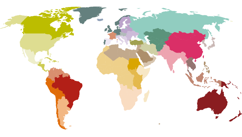
As the various source data series measure disparate phenomena, and are constructed on different scales, a process is required to standardize them for comparison. First, a 90 per cent winsorization is performed to reduce the influence of outliers on the data series. A 90 per cent winsorization sets the bottom 5 per cent of values to the value of the fifth percentile, and sets the top 5 per cent of values to the value of the 95th percentile. Thus countries that are outliers in a data series are not discarded from the dataset (unlike with trimming), but they are limited in their extremity.
Second, a standard minimum-maximum normalization is applied to the winsorized data. This rescales values from their original range and units to a comparable 0–100 scale. The minimum value present in the data is assigned a value of zero, the maximum value is set to 100, and all values in between are proportionally revalued. Min-max normalization captures the best and worst values present in the data, not the theoretical minimum and maximum values attainable. Where necessary, min-max normalized values are inverted so that no matter what the underlying data series, the maximum value (100) always represents the best score present in the data series and the minimum value (0) represents the worst score.
Third, the quartile of each value in the data series is recorded. This provides a rapid intuitive understanding of how any one data point compares with any other, and of how skewness is affecting the data. For example, if there is positive skew (i.e. the mean value is greater than the median), min-max normalized values may be relatively low but still appear in the top quartile. This suggests that although their performance is noticeably inferior to the top performers in the dataset, they still compare relatively well with the majority of the other countries. A high min-max value but a low quartile value suggests the presence of a large number of countries with high min-max values. Thus, the quartile values are most useful for rapidly and crudely considering how a score compares with all other scores in the series, whereas the min-max value gives a better sense of the score relative to the best and worse scores (once extreme outliers have been accounted for). In the full version of the CH-FSD, for each data point we record three values, with the utility of each value depending on the current level and purpose of analysis. These values are:
- the raw value in the native units for the series;
- the winsorized max-min values, displayed on a four-colour gradient, with each colour representing a quarter of the range 0–100; and
- the quartile of each normalized value, displayed on a four-colour gradient, with each colour representing a quartile.